Modern Qiskit, part 2: a simulator is a data structure
Part 1 was about the optimize step. This post takes apart execute: what the primitives actually do with the jobs you hand them, and which simulator to reach for.
The mental model for the whole post is that Aer’s method= option
picks a representation of the quantum state, and every
representation buys a different scaling law:
| method | state object | memory | good for |
|---|---|---|---|
statevector | |ψ⟩, 2ⁿ amplitudes | 16 B · 2ⁿ | exact pure states; the default |
density_matrix | ρ, 2ⁿ×2ⁿ | 16 B · 4ⁿ | exact open-system (noise) — squares the cost |
matrix_product_state | MPS, bond dimension χ | ~ n·χ² | wide but weakly entangled circuits |
stabilizer | tableau, O(n²) bits | polynomial | Clifford-only (Gottesman–Knill) |
So choosing a simulator means matching the representation to the
circuit’s structure — entanglement, Cliffordness, noise — not to its
qubit count. A 500-qubit circuit can be free and a 26-qubit one can be
hopeless, as below. Selection is the same one-liner as always:
Sampler(mode=AerSimulator(method="matrix_product_state")).
Full notebooks are on GitHub.
PUBs, properly: batching and per-job shot counts#
Part 0 used one PUB at a time. The full Sampler PUB is
(circuit, parameter_values, shots), one run() takes a list of
them as a single batched job, and each PUB can override the job-level
shot count:
res = sampler.run([(bell_meas,), (ghz_meas, None, 8192)], shots=1024).result()
print(res[0].data.meas.num_shots, res[1].data.meas.num_shots)   # 1024 8192
On hardware that’s one queue entry for the pair. The parameter_values
slot broadcasts through the Sampler exactly like part 1’s Estimator
sweep — [(pqc, [[0.0], [np.pi]])] returns two result indices from
one PUB, {'0': 1000} and {'1': 1000}. Likewise a single Estimator
PUB can carry a list of observables:
obs = [SparsePauliOp(p) for p in ["ZZ", "XX", "ZI", "XY"]]
est.run([(bell, obs)]).result()[0].data.evs
# array([1.0, 1.0, 0.0132, -0.0391])
⟨ZZ⟩ = ⟨XX⟩ = 1 and the single-qubit and mixed-basis observables are zero to shot noise: the Bell state’s correlations are perfect and its marginals are maximally uninformative.
Precision is a shot budget in disguise#
The Estimator doesn’t take shots; it takes precision, a target
standard error, and returns the achieved bars in data.stds. Asking
for precision=0.01 on ⟨ZZ⟩ under increasing depolarizing noise gave:
| ⟨ZZ⟩ | reported std | √(1−⟨ZZ⟩²) / std |
|---|---|---|
| 0.905 | 0.0043 | 9,950 |
| 0.604 | 0.0080 | 9,970 |
| 0.111 | 0.0099 | 10,000 |
A single ±1 measurement of ZZ has variance 1 − ⟨ZZ⟩², so that last column is the shot count, and it is 10⁴ every time — i.e. Aer solved ε = σ/√N for N = 1/ε². The error bar is constant by construction; the shots are what moves. That’s the trade specifying accuracy instead of budget, and it’s why halving the error bar quadruples runtime.
The degenerate case is worth keeping in mind: ⟨ZZ⟩ on a noiseless Bell
state comes back as 1.0 with stds = 0.0 exactly. The Bell state
is a +1 eigenstate of ZZ, so every shot returns +1 and the sample
variance is identically zero. Shot noise is physics, not a numerical
artifact.
The statevector wall, and where it isn’t#
The default method is exact and exponential: 16 B · 2ⁿ complex amplitudes, all of them, all the time. Timing an n-qubit GHZ expectation value up the range (M1 Pro):
| n | statevector memory | time |
|---|---|---|
| 8 | 0.004 MB | 0.0159 s |
| 10 | 0.016 MB | 0.0112 s |
| 12 | 0.063 MB | 0.0096 s |
| 14 | 0.25 MB | 0.0086 s |
| 16 | 1.0 MB | 0.0074 s |
| 18 | 4.0 MB | 0.0136 s |
| 20 | 16 MB | 0.0309 s |
| 22 | 64 MB | 0.0983 s |
| 24 | 256 MB | 0.4099 s |
The memory column is textbook. The time column is more instructive, because for the first third of it the runtime falls as the problem grows — 8 qubits is slower than 16. Nothing is scaling there except fixed overhead: circuit construction, transpilation, the primitive’s own plumbing. The simulation itself is free at that size, so all you’re timing is Python, with the first iteration warming-up.
Then it turns. The ratio per +2 qubits, which theory says should approach 4:
| n | 16→18 | 18→20 | 20→22 | 22→24 |
|---|---|---|---|---|
| time ratio | 1.8× | 2.3× | 3.2× | 4.2× |
It climbs to 4 only once the exponential clears the overhead floor, somewhere around n = 18. And the last ratio overshoots slightly, which is also expected: a GHZ chain has n−1 CX gates, so the real cost is O(n · 2ⁿ), and the predicted ratio at 22→24 is 4 · (24/22) = 4.4 against 4.2 measured.
The practical lesson is that a scaling law is invisible until it isn’t. Benchmarking this circuit at n ≤ 16 and extrapolating would have shown the method was free. Extending the measured tail instead — ×4 memory and ×4 time per two qubits — gives 26 → 1 GB, 28 → 4 GB, 30 → 16 GB, 32 → 64 GB. Runtime at n = 30 would be under a minute, so it’s RAM that ends the game, not patience. Somewhere in the high twenties the statevector stops fitting.
Noise: predict the number, then measure it#
Noise enters Aer through NoiseModel, you attach the model to the simulator and hand that to a primitive:
nm = NoiseModel()
nm.add_all_qubit_quantum_error(depolarizing_error(p, 2), ["cx"])
est = Estimator(mode=AerSimulator(noise_model=nm, method="density_matrix"))
The two-qubit depolarizing channel E(ρ) = (1−p)ρ + p·I/4 acts once on
the Bell state’s lone CX, and it shrinks every traceless observable by
(1−p). So ⟨ZZ⟩ = 1−p, predictable before running anything. Sweeping p
on both an exact density matrix and statevector + noise (which
unravels the channel into Monte Carlo trajectories, sampling Kraus
operators per shot):
| p | predicted 1−p | density_matrix | trajectories |
|---|---|---|---|
| 0.1 | 0.9 | 0.895 | 0.905 ± 0.004 |
| 0.2 | 0.8 | 0.800 | 0.793 ± 0.006 |
| 0.3 | 0.7 | 0.693 | 0.703 ± 0.007 |
| 0.4 | 0.6 | 0.600 | 0.604 ± 0.008 |
| 0.5 | 0.5 | 0.469 | 0.501 ± 0.009 |
| 0.9 | 0.1 | 0.106 | 0.111 ± 0.010 |
Both columns are the prediction plus sampling noise, which confirms
that Qiskit’s depolarizing_error(p, n) uses exactly the convention
above — worth doing empirically for every noise parameter you meet,
since the factor-of-4 conventions differ between packages.
One thing the table shows that the theory doesn’t: the density-matrix column is not exact either. Its values are all integer multiples of 1/1024. ρ is propagated exactly through the channel, but the Estimator still samples the final expectation value, so “exact simulation” buys you exact channel physics, not an exact number.
Real devices come pre-packaged. NoiseModel.from_backend(FakeManilaV2())
lifts a device’s measured calibration data straight into a model — and
because that data is attached to physical qubits and native gates, it
needs part 1’s ISA plumbing to line up:
isa = pm.run(bell)
est.run([(isa, zz.apply_layout(isa.layout))]).result()   # <ZZ> = 0.896
Manila’s real calibrated error rates cost about 10% of the correlation on a two-qubit circuit.
Readout error is a separate, purely classical animal — a confusion
matrix on the measurement, not a channel on the state. With
p(0→1) = 0.02 and p(1→0) = 0.05, 10,000 Bell shots came back as
{'00': 4773, '11': 4548, '01': 332, '10': 347}. The forbidden
outcomes are 679 shots against 671 predicted from a single flip on
either qubit, and the asymmetry between 00 and 11 is the same
effect: 1s decay to 0s more often than the reverse, so weight drifts
toward 00. No entanglement was harmed, this is entirely a
measurement artifact, which is why it can be mitigated classically.
The circuits that shouldn’t fit#
A 50-qubit GHZ state needs 16 B · 2⁵⁰ ≈ 18 petabytes as a statevector. As a matrix product state it has bond dimension χ = 2, one bit of correlation across any cut, and it samples in a fraction of a second:
s = Sampler(mode=AerSimulator(method="matrix_product_state"))
counts = s.run([ghz_meas(50)], shots=1000).result()[0].data.meas.get_counts()
# {'000...0': 506, '111...1': 494}
That result is fun and almost entirely uninformative, which is worth being explicit about. A GHZ state has χ = 2 at every n, so pushing n higher holds the cost driver fixed and measures overhead. Scaling the qubit count on GHZ can show that MPS is cheap; it structurally cannot show where MPS stops being cheap. To find that, fix n and vary the thing MPS actually pays for.
The catch is that MPS cost tracks entanglement, not width — but demonstrating that takes more care than it looks, because sweeping depth moves two things at once. Each added layer grows entanglement, which is the thing under test; it also adds 38 gates, which would cost more under any representation. A rising MPS curve on its own can’t tell you which of those did it.
So the control is to run the identical circuits under statevector,
which is blind to entanglement by construction, it stores all 2²⁶
amplitudes whether the state is a product state or maximally entangled,
and its cost is gate count and nothing else. A 26-qubit brickwork
circuit, both methods, 100 shots:
| layers | 2 | 10 | 14 | 16 | 17 | 18 |
|---|---|---|---|---|---|---|
matrix_product_state | 0.02 s | 0.03 s | 0.82 s | 4.95 s | 10.0 s | 47.1 s |
statevector | 1.47 s | 7.94 s | 11.4 s | 12.9 s | 14.6 s | 14.8 s |
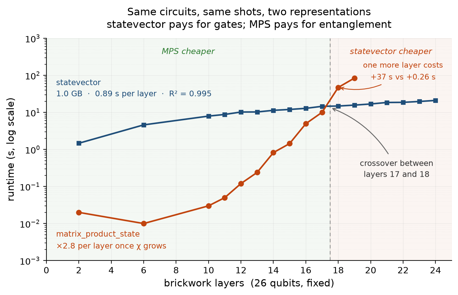
The statevector line is linear, 0.89 s per layer, R² = 0.995 across the whole sweep from 2 to 24 layers, which is exactly the prediction: every gate touches all 1.0 GB of amplitudes, per-gate cost is constant, gate count is linear in depth. That line is the cost of the gates, isolated. MPS climbs by ×2.8 per layer once χ starts moving, and that number is not free-floating: χ doubles every two layers, χ³ therefore grows ×8 every two layers, and 8^(1/2) = 2.83. The measured runtime growth is the staircase, cubed. It pays for entanglement. Every bit of curvature in the MPS line is therefore entanglement and nothing else, which is the claim the experiment was built to support.
Set the two per-gate costs equal and the crossover has a closed form. Statevector costs ~2ⁿ per gate, MPS costs ~χ³, and both apply the same number of gates, so:
χ* ≈ 2^(n/3)
At n = 26 that’s 2^8.67 ≈ 407, against 512 measured. Translate it into depth using the growth law, 2^⌈L/2⌉ = 2^(n/3):
L* ≈ 2n/3
which is 17.3 layers for 26 qubits — the crossover the runtime plot marks between 17 and 18, predicted from nothing but the gate structure and the qubit count.
Keep the two axes distinct while reading that. n is the width and it is fixed at 26 for this entire experiment; L is the depth and it is the swept variable. Depth is what drives χ up. Width does two different jobs: it sets the ceiling χ could ever reach, and it sets the threshold at which MPS stops being worth it.
And MPS loses. The crossover is at layer 17–18: at 17 layers MPS is still ahead, 10.0 s against 14.6 s; one layer later it is 47.1 s against 14.8 s. The marginal cost of that single layer is +37 s on MPS and +0.26 s on statevector, a factor of 140 for the same added gates.
The growth rate has a clean explanation, and it’s worth measuring rather than assuming.
Watching χ itself#
Everything so far infers χ from timings. Aer will simply tell you — though not
through the primitives. SamplerV2’s result[0].metadata carries the shot count
and circuit metadata and nothing else, which is the abstraction doing its job: a
PUB result is meant to be backend-agnostic, and bond dimension is about as
backend-specific as it gets. To see inside the simulator, drop to the Aer backend
directly.
What χ actually is#
Cut the 26-qubit register between site i and site i+1. The amplitudes of the state, re-indexed as (everything left of the cut) × (everything right of the cut), form a matrix. Take its SVD. The singular values are the Schmidt coefficients λₖ, their squares are the eigenvalues of the reduced density matrix, and χ is how many of them are nonzero — the Schmidt rank across that cut. χ = 1 is a product state; larger χ means more entanglement across that particular cut.
A 26-site chain has 25 cuts, so the state carries 25 of these numbers, not one. That matters twice over, because χ plays two roles at once. It is the physics — how entangled is this cut — and it is the invoice: an MPS stores ~n·χ² numbers, and applying a two-qubit gate means SVD-ing the merged pair of site tensors, at a cost of ~χ³. Every claim in this section is one of those two roles talking.
Getting it out of Aer#
qc = brickwork(26, layers)        # no measurements
qc.save_matrix_product_state()
backend = AerSimulator(method="matrix_product_state")
gammas, lambdas = backend.run(qc).result().data()["matrix_product_state"]
chi = [len(l) for l in lambdas]   # Schmidt rank at each of the 25 cuts
Aer returns the state in Vidal canonical form: gammas is one tensor per site,
lambdas is one vector of Schmidt coefficients per cut. So len(l) literally
counts the surviving singular values at that cut — the list comprehension above
is the definition in the previous section, evaluated 25 times.
AerSimulator(..., mps_log_data=True) works too, logging bond dimensions after
every instruction into result.results[0].metadata, but it also has to go through
backend.run(). That’s not a regression to the pre-primitives era: execute() and
Aer.get_backend() are gone, but AerSimulator.run() is live and supported, and
it’s the only route to save instructions — a save_* call has no PUB equivalent.
Either way, note that
Aer applies no bond-dimension truncation by default,
so these are true χ values, not a cap.
Why the staircase is exact#
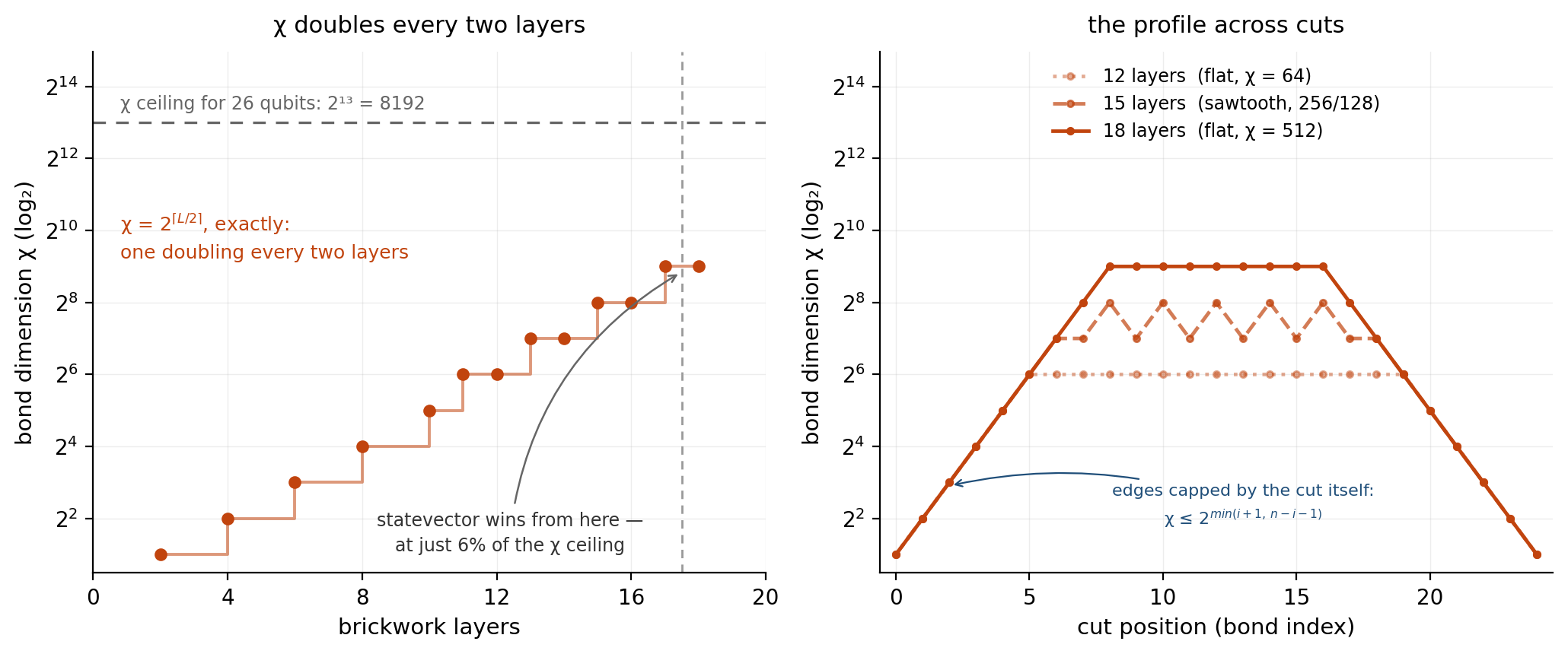
χ = 2^⌈L/2⌉ exactly — 2, 4, 8, 16, 32, … reaching 512 by layer 18. Nothing fitted. Two facts produce that exponent.
First, only a gate that straddles a cut can change χ there. A gate acting entirely on one side is U_A ⊗ I, which sends ρ_A → U_A ρ_A U_A† — a similarity transformation that leaves the eigenvalues of ρ_A untouched. The λ² are those eigenvalues, so the spectrum, and hence the rank, is unchanged. Single-qubit rotations are free as far as χ is concerned; only the entangler counts.
Second, a CX at most doubles χ across the cut it spans. Written as CX = |0⟩⟨0|⊗I + |1⟩⟨1|⊗X it is a sum of two product operators, and a sum of k product operators multiplies the Schmidt rank by at most k. Its operator Schmidt rank is 2.
The brickwork supplies the last ingredient: each bond is straddled on every other layer, so after L layers it has seen ⌈L/2⌉ entanglers. Doubling that many times gives 2^⌈L/2⌉. Note what this is contingent on — a generic (Haar-random) two-qubit gate has operator Schmidt rank 4, which would give 4^⌈L/2⌉ ≈ 2^L and hit the wall in half the depth. The clean power-of-two staircase is a statement about CX-style entanglers, not about brickwork circuits in general.
The profile is the minimum of two curves#
The right panel shows what the peak hides, and it is the product of two independent mechanisms rather than one.
The growth law is what we just derived, and it is uniform across the chain. Brickwork gate density is the same everywhere; there is nothing pyramidal about it, no extra action in the middle.
The cap is geometry. The amplitude matrix at cut i has shape 2^(i+1) × 2^(n−i−1), and a matrix’s rank cannot exceed its smaller dimension, so χ ≤ 2^min(i+1, n−i−1) no matter what circuit you run. That’s a tent peaking at 2¹³ = 8192 in the middle of a 26-qubit chain and collapsing to 2 at the ends.
The measured profile is simply the minimum of the two: a flat line at 2^⌈L/2⌉, clipped near the edges by the tent. The ramp at the shoulders isn’t entanglement growing more slowly out there — it’s the same flat line hitting a ceiling set by where you cut.
The sawtooth is a third, separate feature riding on the flat portion. At odd depth half the bonds have been straddled ⌈L/2⌉ times and half ⌊L/2⌋ times, so the interior alternates between χ and χ/2 — 256/128 at 15 layers. At even depth everyone has caught up and it fills in flat: 64 at 12 layers, 512 at 18.
χ_max is not the cost#
That sawtooth matters more than it looks, because the natural summary statistic is wrong.
Applying a gate at bond i means SVD-ing a matrix of shape (2χ_{i−1}) × (2χ_{i+1}), and SVD of an m×n matrix costs O(m·n·min(m,n)). So the per-gate price is χ_left·χ_right·min(χ_left, χ_right), and the familiar χ³ is only the special case where the profile happens to be flat. Regressing runtime against Σχ³ over the cuts gives a log-log slope of 0.93 with R² = 0.97, so χ³ is the correct cost model across the sweep.
But it under-predicts the one step that stands out: layers 17 and 18 have the same χ_max of 512, yet the runtime quadruples. The sawtooth is why. At depth 17 the interior alternates 512/256, so gates in the next layer mostly contract a 512 bond against a 256 bond; at depth 18 the profile is flat and every gate pays the full 512³. Modelling that layer as Σ χ_left·χ_right·min(χ_left, χ_right) predicts 6.4× against 7.3× measured. The same 4.70× total jump reproduces on two unrelated machines, which is what rules out a cache artifact.
The general lesson survives the brickwork: χ_max is not a sufficient statistic for cost. Any circuit with a non-uniform entanglement profile — a heavy-hex layout, a QAOA instance on an irregular graph — will have the same property, and you need the whole profile to price it.
The number to carry away is 512#
A 26-qubit MPS can hold χ up to 2¹³ = 8192 before it is simply storing the full state — and it never gets close. Statevector overtakes it at 512, about 6% of saturation, right where 2^(n/3) says it should.
That gap isn’t a quirk of this instance; it widens exponentially. The crossover as a fraction of the ceiling is 2^(n/3) / 2^(n/2) = 2^(−n/6) — about 5% at n = 26, about 1% at n = 40. MPS doesn’t fail when entanglement maxes out. It fails when χ³ overtakes 2ⁿ, which happens far earlier, and increasingly so.
(At large n the comparison eventually stops being a contest: 40 qubits is 17.6 TB of statevector, so nothing overtakes anything. Past that point χ* marks where MPS stops being a bargain, not where a better option takes over.)
So MPS is for circuits that are wide but shallow — the DMRG intuition, unchanged — and both words now have numbers attached. Shallow means L < 2n/3 for a rank-2 entangler, half that for a generic one. And the quantity to estimate before reaching for the method is χ against 2^(n/3), not χ against saturation.
Stabilizer: free, or nothing#
The stabilizer tableau is more extreme in both directions. GHZ is Clifford, so Gottesman–Knill applies and 500 qubits is a non-event:
s = Sampler(mode=AerSimulator(method="stabilizer"))
s.run([ghz_meas(500)], shots=100).result()
# 2 distinct outcomes, 51 / 49, in 1.5 s
Add a single qc.t(0) and it refuses to run at all — Aer rejects the
circuit as containing invalid instructions for the method. That is the
whole difference between MPS and stabilizer: entanglement is
continuous, so MPS degrades gracefully and expensively, while
Cliffordness is a yes/no structural property, so stabilizer is either
free or unavailable. One T gate is the entire boundary between
polynomial and exponential, which is also why T-count is the currency
of fault-tolerance costing.
One circuit, four methods#
The deliverable: a 12-qubit hardware-efficient ansatz from part 1, 2
reps, randomly bound parameters, 2048 shots, run under every method.
The Clifford variant swaps each RY/RZ pair for H·S so the circuit
structure is identical but stabilizer-legal. Each method runs in its
own process so ru_maxrss is a per-method peak:
for m in statevector density_matrix matrix_product_state stabilizer; do
    python bench.py "$m"
done
| method | runtime | peak RSS | RSS − baseline |
|---|---|---|---|
| statevector | 0.009 s | 119 MB | ~0 (2¹² amplitudes = 64 kB) |
| density_matrix + depol | 5.06 s | 376 MB | 256.5 MB |
| matrix_product_state | 0.033 s | 122 MB | ~3 MB |
| stabilizer (Clifford) | 0.015 s | 125 MB | ~6 MB |
About 119 MB of every row is the Python process itself, so the deltas are the real content — and the density-matrix delta is the interesting one. 16 B · 4¹² = 256.0 MB. Measured: 256.5 MB. The 4ⁿ object isn’t an asymptotic claim here; it’s sitting in resident memory, agreeing with theory to within half a percent. The other three methods don’t move the needle at all: 12 qubits of statevector is 64 kB, a linear-entangling ansatz keeps χ small, and a tableau is bits.
Extending the memory column is the whole reason to build the table. Density matrix dies first, and fast — 12 → 256 MB, 14 → 4 GB, 15 → 16 GB — so exact noisy simulation on a workstation ends around n ≈ 14–15, roughly half the statevector ceiling from the table earlier, and that’s before the 5 s runtime starts scaling too. Which is the real argument for trajectories: same physics in expectation, 2ⁿ memory instead of 4ⁿ, error bars you can buy down with shots. Against both, the structural methods are unbounded in n and bounded by something else entirely — MPS by entanglement, stabilizer by a single non-Clifford gate.
The practical version, which is the actual takeaway of the phase: reach for statevector by default, density matrix only when you need exact channel physics on a small register (and use trajectories instead the moment n gets awkward), MPS when the circuit is wide and shallow — with “shallow” measured against a statevector control, not assumed — and stabilizer when the circuit is Clifford — where “is it Clifford?” is a question you can answer by reading the gate list, not by benchmarking.
Next up: Phase 3 stops simulating circuits and starts optimizing
them — the Estimator plus scipy.optimize loop that everything since
part 0 has been setting up.