Modern Qiskit, part 1: the compiler is the subject
Part 0 covered the primitives. This post is about the optimize step: what the transpiler does to a circuit on the way to real hardware, and how to measure it. The two numbers that matter throughout are depth (how long the state sits exposed to decoherence) and 2-qubit gate count (2q gates are roughly an order of magnitude noisier than 1q gates on current devices). Everything the compiler does is in service of those two numbers.
Full notebooks are on GitHub.
Circuits as functions: one PUB, whole sweep#
Parameter turns a circuit into a function θ → circuit. The V2
Estimator accepts an entire array of parameter sets inside a single Primitive Unified Bloc
(PUB) — (circuit, observable, parameter_values) — so a sweep is one
batched job rather than a Python loop of bound circuits. On real
hardware that’s one queue entry instead of nine.
Sanity check: a single RY(θ) qubit measured in Z should trace out cos θ. Nine parameter sets through one PUB:
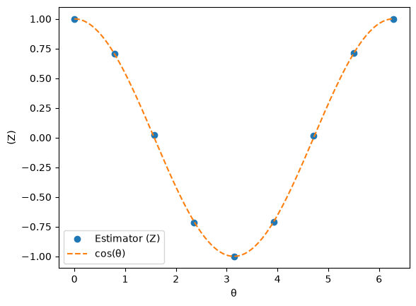
The nine Estimator points land on cos θ to within shot noise (±0.02 at 4096 shots).
A hardware-efficient ansatz, built by hand#
The workhorse variational circuit is layers of parameterized RY·RZ
rotations separated by a fixed CX entangling pattern. I coded it by
hand to follow the parameter bookkeeping, then cross-checked against
the library: for 4 qubits and 2 repetitions, both my hea() and
Qiskit’s efficient_su2 report 24 parameters and 6 CX gates
(2n(reps+1) parameters, as predicted before printing). “Hardware-
efficient” means the entangling pattern is chosen to match a device’s
coupling map rather than the problem — a claim the next section puts
to the test.
The benchmark: entangling pattern vs. topology#
The experiment: transpile two 5-qubit, 2-rep ansatz that differ
only in entangling pattern — linear (a chain, matching real
device connectivity) and full (all-to-all, fighting it) — at every
optimization level, against two device snapshots. seed_transpiler=42
throughout, since layout and routing are stochastic. Entries are
depth / 2-qubit gates.
FakeManilaV2 — 5 qubits in a line, CX-native:
| ansatz | raw | level 0 | level 1 | level 2 | level 3 |
|---|---|---|---|---|---|
| linear | 14 / 8 | 26 / 8 | 23 / 8 | 23 / 8 | 23 / 8 |
| full | 20 / 20 | 76 / 74 | 66 / 61 | 68 / 45 | 68 / 45 |
FakeSherbrooke — 127 qubits, heavy-hex, ECR-native:
| ansatz | raw | level 0 | level 1 | level 2 | level 3 |
|---|---|---|---|---|---|
| linear | 14 / 8 | 80 / 8 | 47 / 8 | 33 / 8 | 33 / 8 |
| full | 20 / 20 | 366 / 74 | 192 / 65 | 190 / 47 | 190 / 47 |
What the tables say:
Linear never pays a routing cost. Its 2q count is 8 before and after, on both devices, at every level — the entangling pattern is already a sub-path of both coupling maps, so routing has nothing to do. The depth still grows because translation rewrites RY/RZ pairs into the native gate set. That’s “hardware-efficient” made visible.
Full gets routed, hard. 20 native CX become 45–74 physical 2-qubit gates: every inserted SWAP costs 3 CX, and an all-to-all pattern on a line (or a heavy-hex lattice) needs a lot of them. On a real device, doubling or tripling the noisy-gate budget is the difference between signal and mush.
Optimization levels buy real reductions — with a trade-off. On Manila, going from level 1 to level 2 cuts the full ansatz’s 2q count from 61 to 45 while the depth ticks up from 66 to 68: the optimizer resynthesized blocks into fewer, differently-arranged 2q gates. Since 2q error dominates, that’s usually the right trade. Levels 2 and 3 tie here because the circuit is small; their gap opens on larger circuits.
Basis gates matter as much as connectivity. Sherbrooke’s depths dwarf Manila’s even for the routing-free linear ansatz (33 vs. 23 at best) because its native 2q gate is ECR — every CX decomposes into an ECR plus single-qubit corrections. A circuit’s cost is a property of the (circuit, target) pair, not the circuit alone.
The glue for variational loops: apply_layout#
After transpiling, virtual qubit i lives on some physical qubit, so an observable written for the virtual circuit is aimed at the wrong wires. Transpiling my 4-qubit ansatz for Manila keeps all 24 parameters free, and remapping the observable is one line:
isa = pm.run(ansatz)                    # still 24 free parameters
isa_obs = obs.apply_layout(isa.layout)  # ZZZZ -> IZZZZ (5 physical qubits)
With all angles set to 0 the state is |0000⟩ and the Estimator
returns ⟨ZZZZ⟩ = 1.0 — the sanity check passes. The pattern for every
variational loop ahead: transpile the ansatz once (it stays
parameterized), remap the observable once, then iterate only over
parameter values via PUBs. Forgetting apply_layout raises no error;
it just silently measures the wrong physical qubits — the nastiest
bug class in hybrid algorithms, which is exactly why the θ = 0 check
is worth automating as a test.
Interop: parameters survive QASM3#
OpenQASM 3 is the interchange format between SDKs, and unbound parameters round-trip through it as typed inputs:
OPENQASM 3.0;
include "stdgates.inc";
input float[64] theta;    // the free parameter, preserved
qasm3.loads() restores the circuit with its parameter intact
(OpenQASM 2 can’t express one at all — the exporter raises). That’s
the escape hatch for moving circuits toward Cirq or CUDA-Q later in
the series.
Next up: taking the execute step apart — statevector, density matrix, MPS, and stabilizer simulation, and where each one’s scaling wall sits.