Modern Qiskit, part 0: primitives and the patterns workflow
This is the first post in a series working through the modern Qiskit
stack (Qiskit 2.4.2, qiskit-aer 0.17.2, qiskit-ibm-runtime 0.47.0,
Python 3.12). Qiskit’s 0.x → 1.0 → 2.x transition removed most of what
older tutorials teach — execute(), opflow, qiskit.algorithms are
all gone — so the series sticks strictly to the current model: every
program is map → optimize → execute → analyze, and execution goes
through the V2 primitives. Everything below runs locally on
AerSimulator through the runtime primitives; the same code targets
real hardware by swapping the backend, which is the point of the
primitives design.
Full notebooks are on GitHub.
Sampler: distributions over bitstrings#
SamplerV2 answers “what did I measure, and how often?” — so its
circuits must contain measurements. The hello-world case is a Bell
state:
bell = QuantumCircuit(2)
bell.h(0)
bell.cx(0, 1)
bell.measure_all()

sampler = Sampler(mode=AerSimulator())
result = sampler.run([bell], shots=4096).result()
result[0].data.meas.get_counts()   # {'00': 2026, '11': 2070}
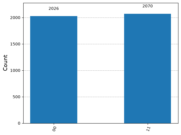
Only 00 and 11 ever appear, split 2026/2070 over 4096 shots — the
qubits are perfectly correlated, never independent.
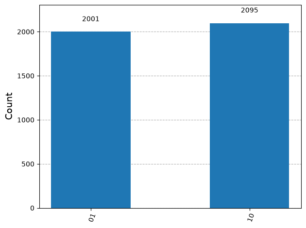
Prepending an X gate before the entangler prepares |Ψ⁺⟩ = (|01⟩ + |10⟩)/√2 instead, and the histogram flips to the anti-correlated outcomes:
Estimator: expectation values, and why it’s a separate primitive#
EstimatorV2 answers “what is ⟨ψ|O|ψ⟩?” directly. You hand it an
observable as a SparsePauliOp and a circuit without measurements;
it handles the basis rotations and averaging internally. On the Bell
state it returns ⟨ZZ⟩ = 1.0. The state |Φ⁺⟩ is a +1 eigenstate of ZZ.
The more interesting check is on |Ψ⁺⟩, in two bases:
for label in ["ZZ", "XX"]:
    obs = SparsePauliOp(label)
    result = estimator.run([(psiplus, obs)]).result()
    print(label, float(result[0].data.evs))
# ZZ -1.0
# XX  1.0
That pair of numbers is the difference between entanglement and mere
classical correlation. A classical 50/50 mixture of 01 and 10 also
gives ⟨ZZ⟩ = −1, but its ⟨XX⟩ is 0. Getting ⟨XX⟩ = +1 as well means the
correlations survive a change of basis — only the coherent
superposition does that.
It also explains why Sampler and Estimator coexist. You could compute ⟨ZZ⟩ from Sampler counts by hand, but X- and Y-basis observables need basis-change circuits, and Estimator does all of that for you, with proper error bars. The variational algorithms later in this series (VQE, QAOA) are “minimize an expectation value,” so Estimator is their native interface; Sampler is for when the bitstrings themselves are the answer, like reading out a QAOA solution. Different questions, different primitives.
GHZ, and a first look at the compiler#
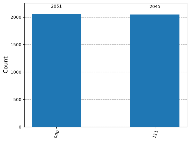
Extending to a 3-qubit GHZ state gives the expected two-outcome histogram — 2051/2045 over 4096 shots:
Before running, I also pushed the GHZ circuit through
generate_preset_pass_manager against FakeManilaV2, a snapshot of a
real 5-qubit IBM device. The depth grew from 3 to 5 while the 2-qubit
gate count stayed at 2, and the layout mapped virtual qubits straight
onto physical qubits 0–2 — the circuit already fit Manila’s line
topology, so the growth came purely from translating into the device’s
native gate set. Circuits that don’t fit the topology pay a much
steeper price, which will be tested next in
part 1 of this series.